
Pandas is an open source library providing high-performance, easy-to-use data structures and data analysis tools for the Python programming language. Pandas is the most popular python library that is used for data analysis.
Key Features of Pandas:
- Fast and efficient DataFrame object with default and customized indexing.
- Tools for loading data into in-memory data objects from different file formats.
- Data alignment and integrated handling of missing data.
- Reshaping and pivoting of date sets.
- Label-based slicing, indexing and subsetting of large data sets.
- Columns from a data structure can be deleted or inserted.
- Group by data for aggregation and transformations.
- High performance merging and joining of data.
- Time Series functionality.
Install and import Pandas:
If you install Anaconda Python package, Pandas will be installed by default.
Also you can install through your terminal window either of the following commands:
conda install pandasOr via PyPI:
pip install pandasImport pandas library:
# Import Panda Library
import pandas as pd
Data analysis with Pandas:
We can analyze data in pandas with following two primary components:
- Series
- DataFrame
Series:
Series is one-dimensional (1-D) labeled array capable of holding any data type.
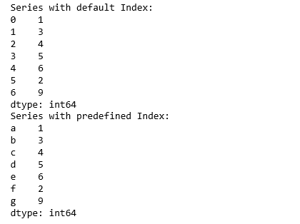
Creating series with basic data collection and index:
# Numeric data collection
Data =[1, 3, 4, 5, 6, 2, 9]

# Creating series with default index values
sr1 = pd.Series(Data)

print("Series with default Index:")
print(sr1)

# Predefined index values
Index =['a', 'b', 'c', 'd', 'e', 'f', 'g']

# Creating series with predefined index values
sr2 = pd.Series(Data, Index)

print("Series with predefined Index:")
print(sr2)
Output:
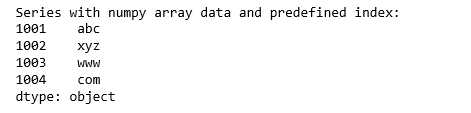
Creating series from Numpy array:
# Import Numpy Library
import numpy as np

# Numpy array data collection
data = np.array(['abc','xyz','www','com'])

# Predefined index values
index=[1001,1002,1003,1004]

# Creating series with numpy array data and predefined index values.
sr3 = pd.Series(data,index)

print("Series with numpy array data and predefined index:")
print(sr3)
Output:
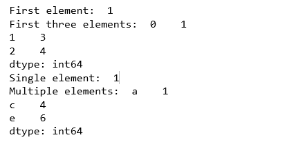
Retrieving data from Series object:
#retrieve the first element.
print('First element: ', sr1[0])

#retrieve the first three element.
print('First three elements: ', sr1[:3])

#retrieve a single element.
print('Single element: ', sr2['a'])

#retrieve multiple elements.
print('Multiple elements: ', sr2[['a','c','e']])
Output:
DataFrame:
DataFrame is two-dimensional (2-D) data structure defined in pandas which consists of rows and columns.
In general, Pandas DataFrame consists of three main components: the data, the index, and the columns.
Creating DataFrame from simple data collection
Let’s create a data structure for employee records. Following table represent the employee data.
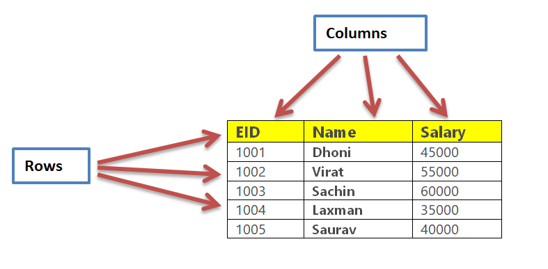
Creating DataFrame based on above employee table.
# Employee data collection.
data = {
    'EID': [1001, 1002, 1003, 1004, 1005],
    'Name': ['Dhoni', 'Virat', 'Sachin', 'Laxman', 'Saurav'],
    'Salary': [45000, 55000, 60000, 35000, 40000]
}

# Create DataFrame based on the employee data collection with index.
empDataFrame = pd.DataFrame(data, index=['rank1','rank2','rank3','rank4', 'rank5'])

empDataFrame
Output:

Reading data from CSV file
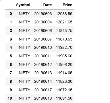
Creating DataFrame from CSV file. Let’s fetch Nifty Index price sheet for month of June and draw a price chart.
Date Source: CSV file.
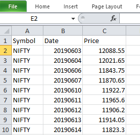
Reading CSV file into DataFrame.
import pandas as pd

# Input file name.
inputFilename = r'''F:\PURNA\AI_ML\Python\NumpyPandas\NiftyPriceSheetJune2019.csv'''

# Read the CSV file through read_csv() function
dframe = pd.read_csv(inputFilename)

dframe
Output:
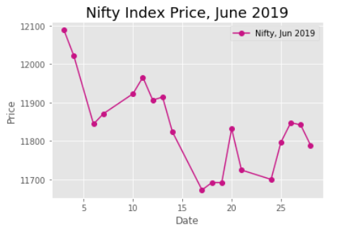
Creating Stock price line chart from DataFrame above.
# Import Matplotlib Library
from matplotlib import pyplot as plt

plt.style.use('ggplot')

# plot with matplotlib
plt.plot( 'Date', 'Price', data=dframe, marker='o', color='mediumvioletred')
plt.ylabel('Price')
plt.xlabel('Date')

plt.title('Nifty Index Price, June 2019', fontsize='18')
plt.legend(['Nifty, Jun 2019'], loc=1)

plt.show()
Output:
To be continued..
Reference Source:

Leave a comment