
We covered a lot on basics of pandas in Python – Introduction to the Pandas Library, please read that article before start exploring this one.
DataFrame is two-dimensional (2-D) data structure defined in pandas which consists of rows and columns. Each column in a DataFrame is a Series object, rows consist of elements inside Series.
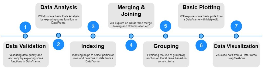
We will explore the Olympics dataset using Pandas DataFrame in this article.
Reading data from CSV file:
Read the Olympics dataset from CSV file into DataFrame.
# Import Pandas library.
import pandas as pd

# Read the olympics dataset from CSV file.
df = pd.read_csv('data/olympics_athlete_events.csv')  # You can also skips rows using skiprows=4
1. Data validation:
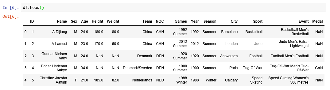
head() and tail():
head() – Return the first 5 rows by default.
head(2) – Return the first 2 rows as specified.
tail() – Return the last 5 rows by default.
tail(2) – Return the last 2 rows as specified.
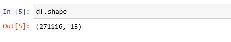
shape:
Return the dimensions of the DataFrame.
info():
Print a concise summary of a DataFrame.
This method prints information about a DataFrame including the index dtype and column dtypes, non-null values and memory usage.
describe():
Generate descriptive statistics that summarize the central tendency, dispersion and shape of a dataset’s distribution, excluding NaN values.
print("Shape of the DataFrame: ", df.shape)

print("Head of the DataFrame: ", df.head())
print("Head of the DataFrame with two records: ", df.head(2))

print("Tail of the DataFrame: ", df.tail())
print("Tail of the DataFrame with two records:: ", df.tail(2))

print("Information about DataFrame: ", df.info())

print("Describe the DataFrame: ", df.describe())
2. Basic Data Analysis:
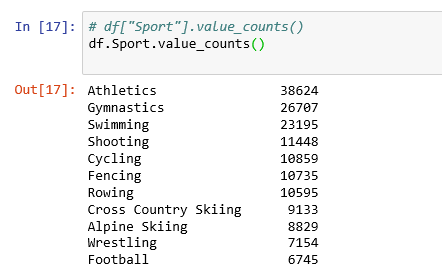
value_counts():
Return a Series containing counts of unique values.
# df["Sport"].value_counts()
df.Sport.value_counts()
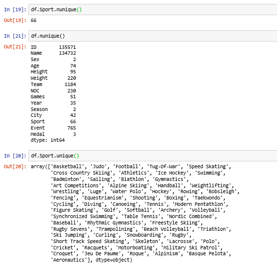
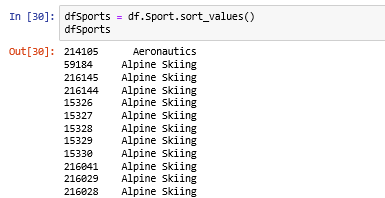
unique() and nunique():
unique() – Return unique values of column or series.
nunique() – Return the number of unique elements in the column or series.
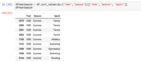
sort_values():
Series.sort_values() – Sort by the values from series object.
DataFrame.sort_values() – Sort by the values from dataframe along with columns.
Sorting on Series.
Sorting on DataFrame.
Source code:
dfSports = df.Sport.sort_values()
dfSports

dfYearSeason = df.sort_values(by=['Year','Season'])[['Year','Season', 'Sport']]
dfYearSeason
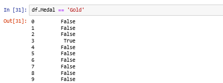
Boolean indexing:
In Boolean Indexing, Boolean Vectors can be used to filter the data. Multiple conditions can be grouped in brackets.
Let’s take a condition where we will filter out all the data in which the athletes have won the Gold Medal.
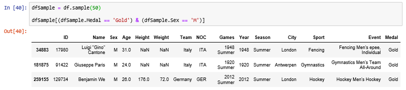
Let’s filter the data in which male athletes have won Gold medal from a sample of 50 records.
Source code:
df.Medal == 'Gold'

dfSample = df.sample(50)
dfSample[(dfSample.Medal == 'Gold') & (dfSample.Sex == 'M')]
Filter data frame with in a list:
Pandas isin() method is used to filter data frames. isin() method helps in selecting rows with having a particular(or Multiple) value in a particular column.
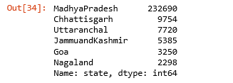
selected_states = ['MadhyaPradesh', 'Chhattisgarh', 'Uttaranchal', 'JammuandKashmir','Goa', 'Nagaland']
dfEventMap = dfEvent[dfEvent["state"].isin(selected_states)]
dfEventMap["state"].value_counts()
Output:
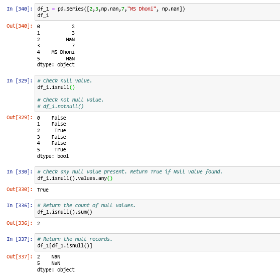
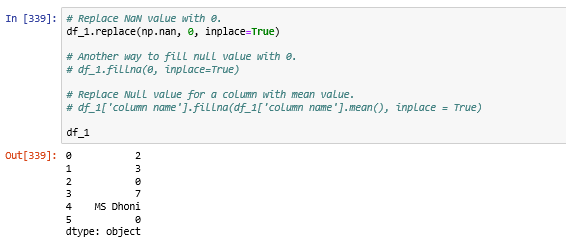
Handling NaN (Null) value in data frame:
Drop Null value in data frame:
df.dropna(inplace=True)Replacing Null value with specific value:
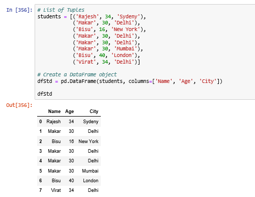
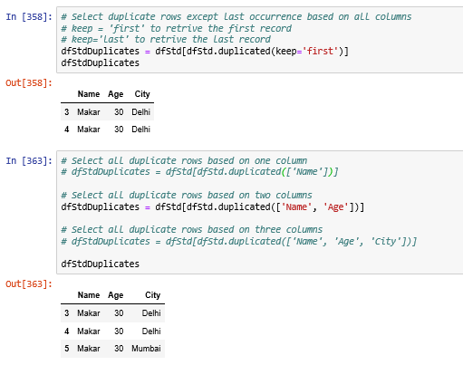
Find Duplicate Rows based on selected columns or all columns:
Created a dataframe for handling duplicates operation.
Find duplicate rows based on one column or multi column or rows:
String handling:
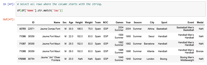
Select all rows where the column starts with the string.
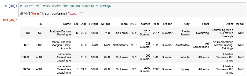
Select all rows where the column contain a string.
Converting a column data type to string and do some operation.
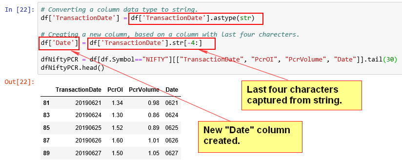
Source code:
# Select all rows where the column starts with the string.

df[df['Name'].str.match('Jau')]

# Select all rows where the column contain a string.

df[df['Name'].str.contains('singh')]
Applying a function on DataFrame:
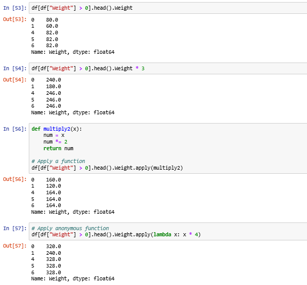
We can apply a function on the column of the DataFrame.
Source code:
df[df["Weight"] > 0].head().Weight

df[df["Weight"] > 0].head().Weight * 3

# Create a function
def multiply2(x):
    num = x
    num *= 2
    return num

# Apply a function
df[df["Weight"] > 0].head().Weight.apply(multiply2)

# Apply anonymous function
df[df["Weight"] > 0].head().Weight.apply(lambda x: x * 4)
3. Indexing:
Indexing help us to select particular rows and columns of data from a DataFrame.
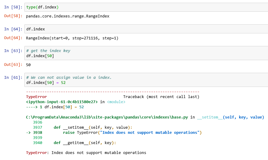
index:
An index is the row label in the DataFrame.
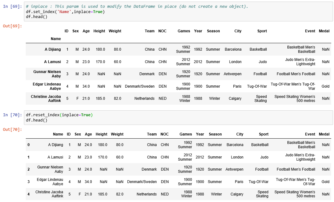
set_index() and reset_index():
set_index(): Set the DataFrame index using existing columns.
reset_index() : Reset the index of the DataFrame, and use the default one instead.
inplace : This param is used to modify the DataFrame in place (do not create a new object).
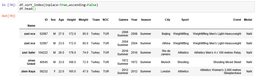
sort_index():
Sorting DataFrame object by index column.
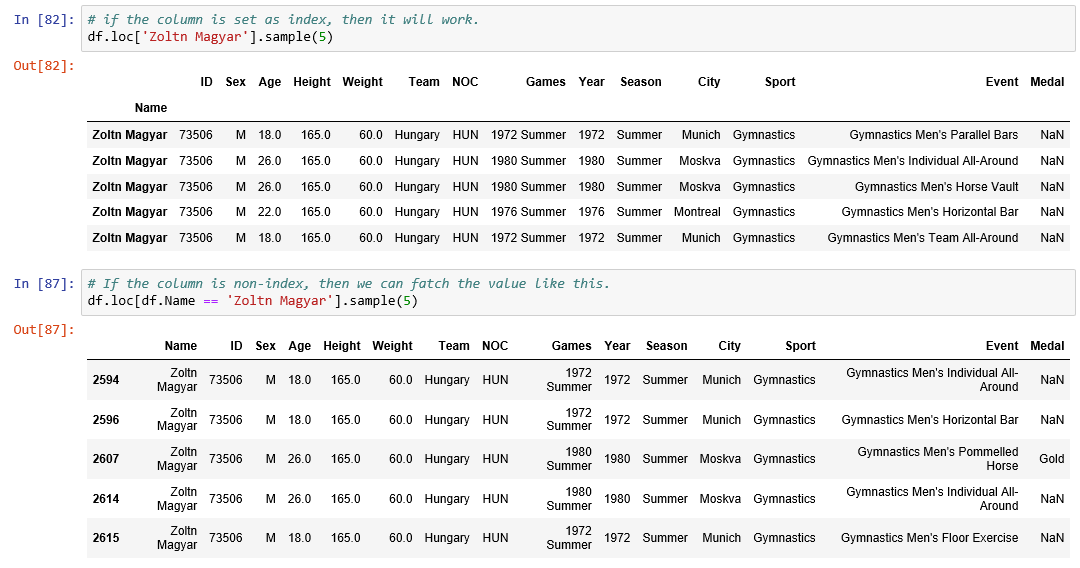
loc and iloc:
Use .loc[] to choose rows and columns by label.
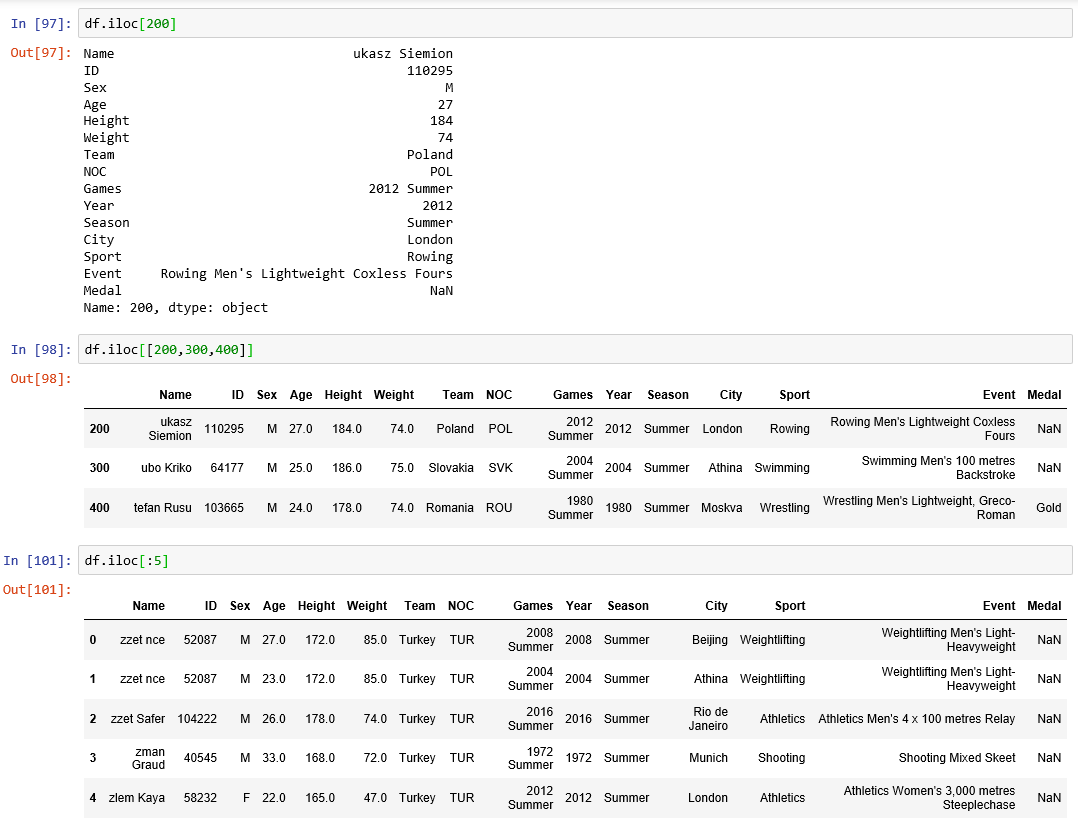
Use .iloc[] to choose rows and columns by position.
Purely integer location based indexing for selection by position.
We can also play with index position using Boolean indexing.
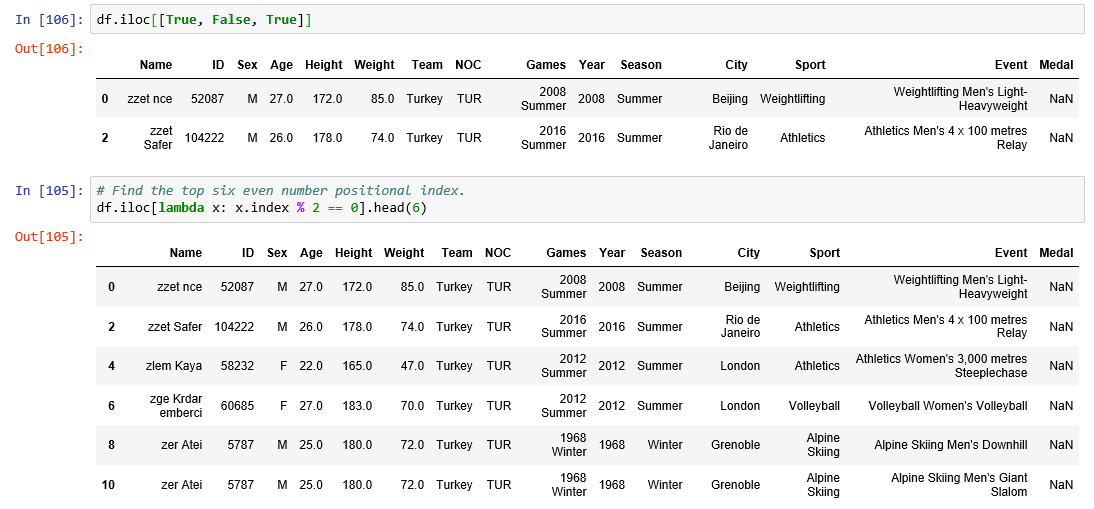
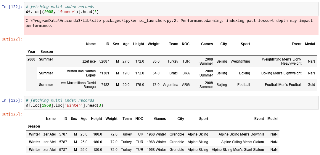
Fetching multi index data.
4. Merging, Joining & Alter Columns:
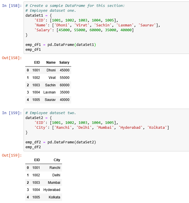
Create two DataFrame from sample dataset. We will use these throughout this section.
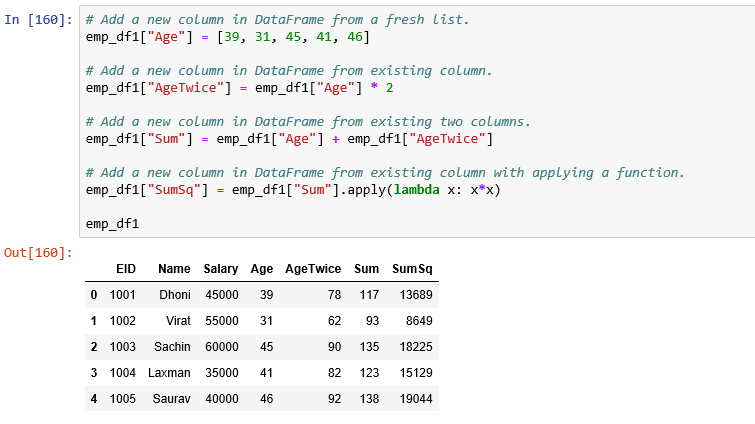
Add Column in DataFrame:
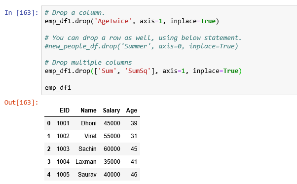
Delete Column in DataFrame:
Column deletion in DataFrame using drop function. It has 2 parameters axis and inplace.
- axis=1 implies delete column wise,
- axis=0 implies delete rowwise
- inplace=True implies Modify the DataFrame
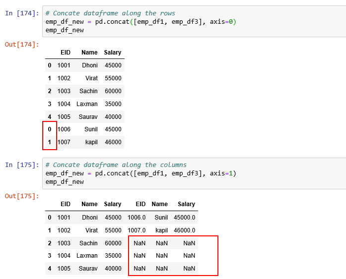
Concatenating two Dataframes:
Create another DataFrame.
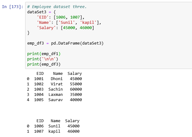
Concatenate DataFrames based on Rows and Columns.
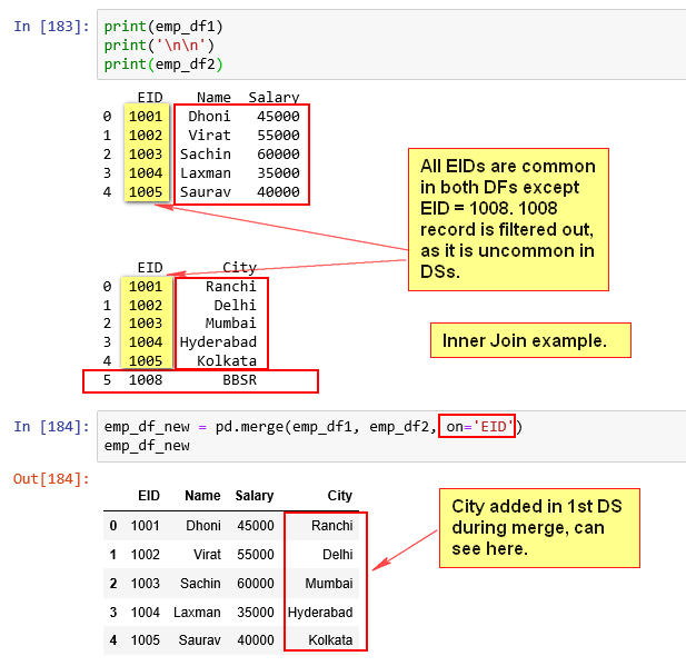
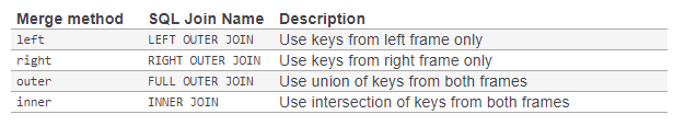
Merging DataFrames:
Merge two DataFrames along the EID value.
Inner Join example.
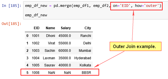
Outer Join example.
Merge method as SQL meaning.
Joining DataFrames:
Index must needed to perform Join in pandas.

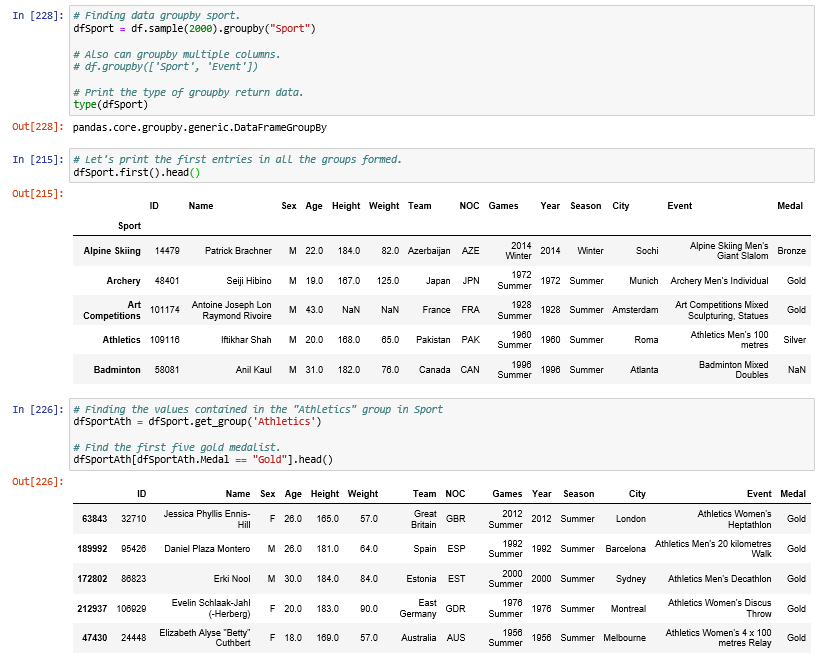
5. Grouping:
Pandas groupby() function is used to split the data into groups based on some criteria.
By “group by” we are referring to a process involving one or more of the following steps:
- Splitting the data into groups based on some criteria.
- Applying a function to each group independently.
- Combining the results into a data structure.
Applying multiple functions to columns in groups.
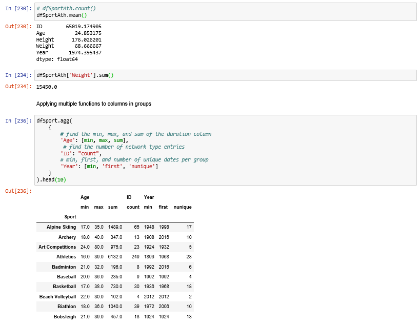
Multiple statistics per group:
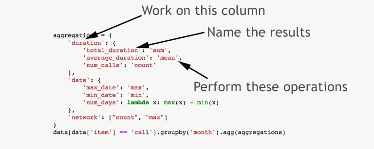
Aggregation of variables in a Pandas Dataframe using the agg() function.
Create CSV file from data frame:
The to_csv() function used to write object to a comma-separated values (csv) file.
dfEventMap.to_csv(r'data\events_data_filtered_tableau.csv', index = False)
6. Basic Plotting:
A picture is worth a thousand words, and we can draw plots with Python’s Pandas and matplotlib library.
Plot():
The only real pandas call we’re making here is ds.plot(). This calls plt.plot()internally.
Make plots of DataFrame using matplotlib / pylab.
When you use .plot on a dataframe, you sometimes pass things to it and sometimes you don’t.
.plot plots the index against every column .plot(x='col1') plots against a single specific column .plot(x='col1', y='col2') plots one specific column against another specific column.
Here are the kind of Plots we can draw.
kind : str
‘line’ : line plot (default)
‘bar’ : vertical bar plot
‘barh’ : horizontal bar plot
‘hist’ : histogram
‘box’ : boxplot
‘kde’ : Kernel Density Estimation plot
‘density’ : same as ‘kde’
‘area’ : area plot
‘pie’ : pie plot
‘scatter’ : scatter plot
‘hexbin’ : hexbin plot
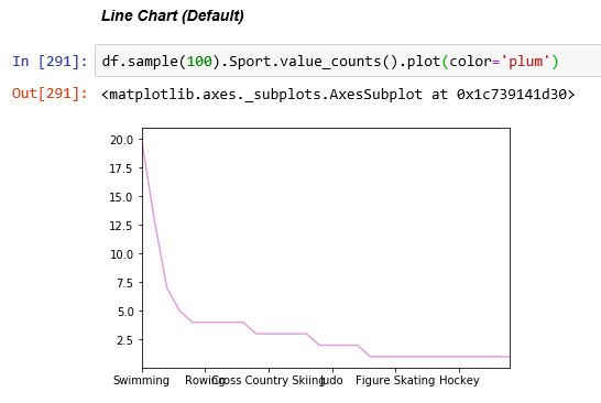
Line Chart (Default):
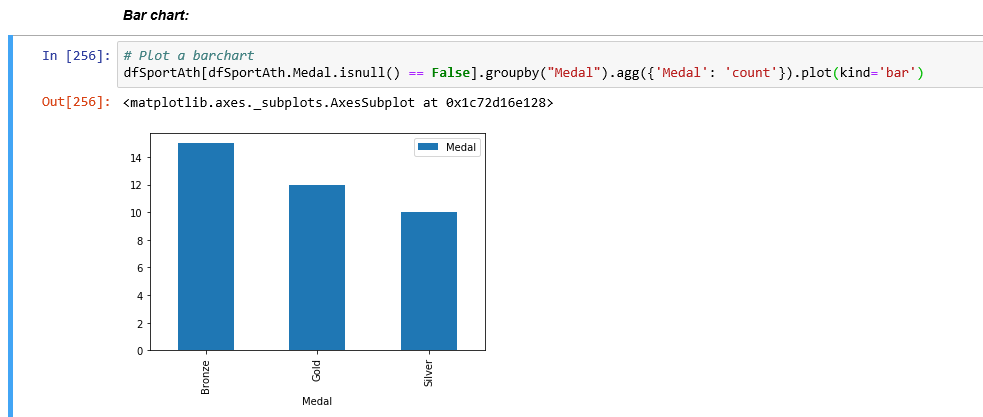
Bar chart:
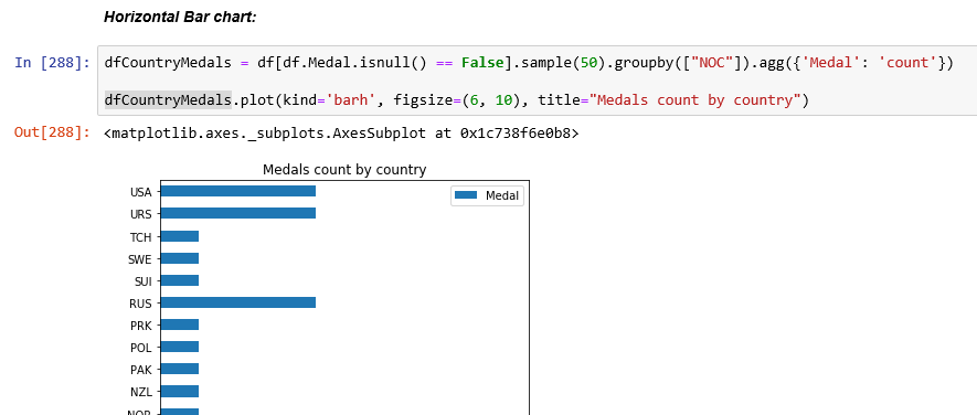
Horizontal Bar chart:
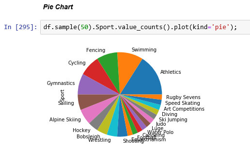
Pie Chart:
7. Data Visualization:
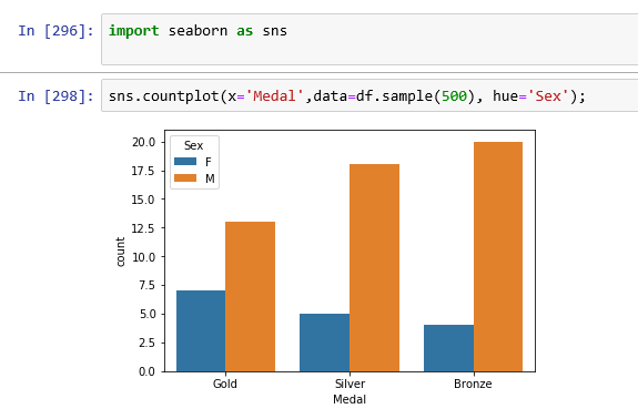
Bar Chart:
Let’s plot a bar chart using Seaborn.
import seaborn as sns;

sns.countplot(x='Medal',data=df.sample(500), hue='Sex');
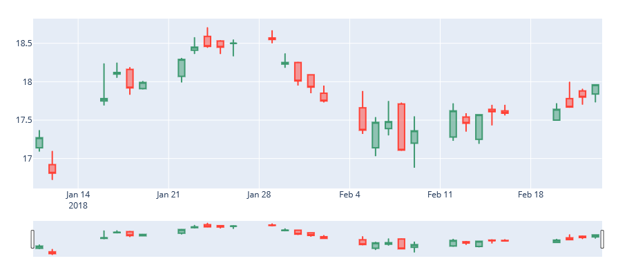
Candlestick Chart:
A candlestick chart shows the open, high, low, and close prices for an asset. The color and positioning of each new candle indicates the price trend.
Let’s plot a candlestick chart using Plotly.
# Install plotly library
!pip install plotly
# Import required packages.
import pandas as pd
import plotly.graph_objects as go
from datetime import datetime
# Create a Dataset for a stock, including symbol, date, low, high, open, and close.
data = {
    "symbol": "XYZ",
    "date": ["2018-01-11", "2018-01-12", "2018-01-16", "2018-01-17", "2018-01-18", "2018-01-19", "2018-01-22", "2018-01-23", "2018-01-24", "2018-01-25", "2018-01-26", "2018-01-29", "2018-01-30", "2018-01-31", "2018-02-01", "2018-02-02", "2018-02-05", "2018-02-06", "2018-02-07", "2018-02-08", "2018-02-09", "2018-02-12", "2018-02-13", "2018-02-14", "2018-02-15", "2018-02-16", "2018-02-20", "2018-02-21", "2018-02-22", "2018-02-23"],
    "low": [17.09, 16.719999, 17.690001, 18.049999, 17.83, 17.9, 17.99, 18.360001, 18.440001, 18.360001, 18.33, 18.5, 18.18, 17.950001, 17.85, 17.73, 17.32, 17.030001, 17.299999, 17.1, 16.879999, 17.23, 17.35, 17.190001, 17.43, 17.559999, 17.5, 17.66, 17.700001, 17.73],
    "high": [17.370001, 17.1, 18.24, 18.25, 18.190001, 18.01, 18.309999, 18.58, 18.709999, 18.540001, 18.549999, 18.67, 18.370001, 18.26, 18.09, 17.950001, 17.879999, 17.540001, 17.75, 17.73, 17.549999, 17.719999, 17.59, 17.57, 17.700001, 17.700001, 17.719999, 18, 17.91, 17.959999],
    "open": [17.139999, 16.92, 17.75, 18.1, 18.16, 17.91, 18.07, 18.41, 18.59, 18.530001, 18.5, 18.57, 18.23, 18.25, 18.09, 17.85, 17.66, 17.139999, 17.389999, 17.709999, 17.200001, 17.280001, 17.540001, 17.25, 17.639999, 17.620001, 17.5, 17.780001, 17.879999, 17.84],
    "close": [17.27, 16.809999, 17.780001, 18.120001, 17.92, 17.99, 18.290001, 18.450001, 18.459999, 18.450001, 18.5, 18.549999, 18.25, 18.01, 17.93, 17.75, 17.370001, 17.469999, 17.48, 17.110001, 17.360001, 17.620001, 17.459999, 17.57, 17.610001, 17.59, 17.639999, 17.67, 17.799999, 17.959999]
}

# Create a DataFrame based on the dataset above.
df = pd.DataFrame(data)

# Prepare the candlestick chart.
fig = go.Figure(data=[go.Candlestick(x=df['date'],
                open=df['open'],
                high=df['high'],
                low=df['low'],
                close=df['close'])])

# Show the plot.
fig.show()
Output:
All the source code used in this article can be find in the link here.

To be continued..

Leave a comment