Purnananda Behera

What is Regression?

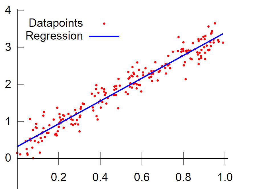
Regression searches for relationships among variables.

Regression is a method for studying the relationship between two or more quantitative variables.

Regression analysis is a form of predictive modelling technique which investigates the relationship between a dependent and independent variable.

For example, you can observe several employees of some company and try to understand how their salaries depend on the features, such as experience, level of education, role, city they work in, and so on.

This is a regression problem where data related to each employee represent one observation. The presumption is that the experience, education, role, and city are the independent features, while the salary depends on them.

What is Linear Regression?

It is a linear model that establishes the relationship between a dependent variable y(Target) and one or more independent variables denoted X(Inputs).

It is a linear approach to

• modeling the relationship between
• a response (or dependent variable) and
• one or more explanatory variables (or independent variables).

The case of one explanatory variable is called simple linear regression. For more than one explanatory variable, the process is called multiple linear regression.

Some Regression Terms:

Multicollinearity: The situation where the explanatory variables are highly inter-correlated is referred to as multicollinearity.

Predicted Values: Predicted, or fitted, values are values of y predicted by the least squares regression line obtained by plugging in x1,x2,…,xn into the estimated regression line.

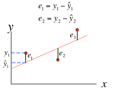
Residuals: Residuals are the deviations of observed and predicted values.

Correlation and Causation:

Correlation helps us determine the degree of relationship between two or
more variables, it does not tell about the cause and effect relationship.

Correlation does not imply causation though the existence of
causation always implies correlation.

Let’s understand this better with examples.

• Cigarette causes cancer – example of causation
• Cigarette smokers also drink alcohol – example of correlation

Simple Linear Regression

Simple linear regression (SLR):
One quantitative dependent variable
– response variable
– dependent variable
– Y
One quantitative independent variable
– explanatory variable
– predictor variable
– X

Linear regression is a basic and commonly used type of predictive analysis. The overall idea of regression is to examine two things:

• Does a set of predictor variables do a good job in predicting an outcome (dependent) variable?
• Which variables in particular are significant predictors of the outcome variable, and in what way they do impact the outcome variable?

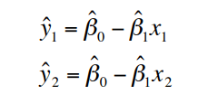
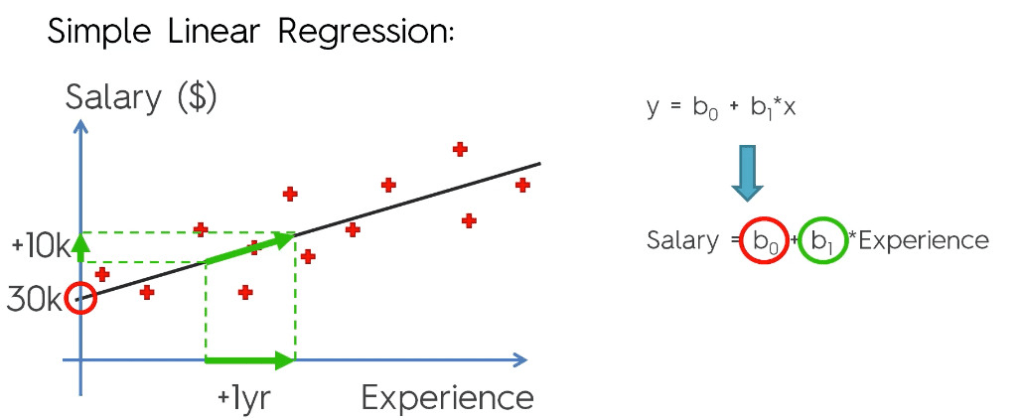
These regression estimates are used to explain the relationship between one dependent variable and one or more independent variables. The simplest form of the regression equation with one dependent and one independent variable is defined by the formula :
𝑦=𝛽0+𝛽1𝑥y=β0+β1x

In this part, you will understand and learn how to implement the Simple Linear Regression models:

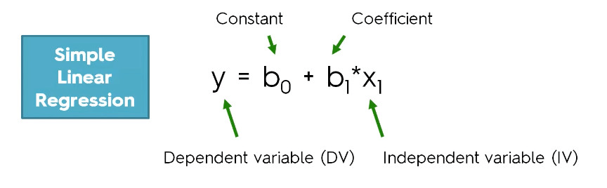
The constant term in regression analysis is the value at which the regression line crosses the y-axis.The constant is also known as the y-intercept.

The intercept (often labeled the constant) is the expected mean value of Y when all X=0.

Regression coefficients represent the mean change in the response variable for one unit of change in the predictor variable while holding other predictors in the model constant.

The key to understanding the coefficients is to think of them as slopes, and they’re often called slope coefficients.

lets do some programming on Sample Linear Regression:

Importing the libraries

# Importing the libraries
import numpy as np
import matplotlib.pyplot as plt
import pandas as pd

# Importing the sklearn libraries to train and test and to perform linear regression. 
from sklearn.model_selection import train_test_split
from sklearn.linear_model import LinearRegression

Importing the dataset

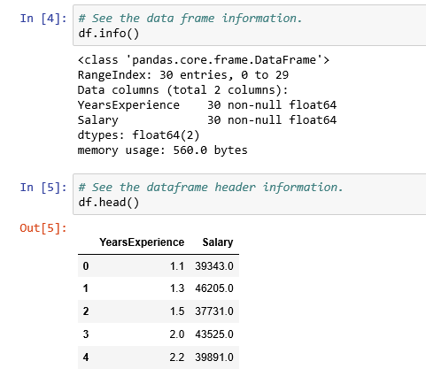
Here we are using a salary dataset having two columns YearsExperience and Salary for our programming practice.

# Importing the dataset
df = pd.read_csv('../Data/Salary_Data.csv')

Validate the dataset

Preparing data for X and Y from Dataframe

X = df.iloc[:, :-1].values
y = df.iloc[:, 1].values

Splitting X and y into training and test dataset

# Splitting the dataset into the Training set and Test set
X_train, X_test, y_train, y_test = train_test_split(X, y, test_size = 1/3, random_state = 0)

Fitting Simple Linear Regression to the Training set

# Fitting Simple Linear Regression to the Training set
linreg = LinearRegression()
linreg.fit(X_train, y_train) 

Predicting the Test set results

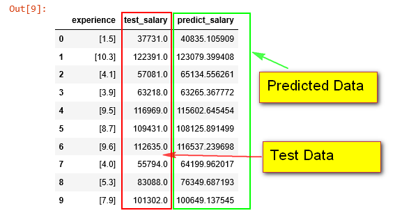
# Predicting the Test set results
y_pred = linreg.predict(X_test)

df_sample = pd.DataFrame({'experience': X_test.tolist(), 'test_salary': y_test, 'predict_salary': y_pred})
# print(X_test, y_test, y_test)

df_sample

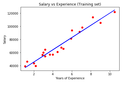
Visualising the Training set results

# Visualising the Training set results
plt.scatter(X_train, y_train, color = 'red')
plt.plot(X_train, linreg.predict(X_train), color = 'blue')
plt.title('Salary vs Experience (Training set)')
plt.xlabel('Years of Experience')
plt.ylabel('Salary')
plt.show()

Visualising the Test set results

# Visualising the Test set results
plt.scatter(X_test, y_test, color = 'red')
plt.plot(X_train, linreg.predict(X_train), color = 'blue')
plt.title('Salary vs Experience (Test set)')
plt.xlabel('Years of Experience')
plt.ylabel('Salary')
plt.show()

How Good Is Your Model?

There are three metrics widely used for evaluating linear model performance.

• R-squared
• RMSE
• MAE

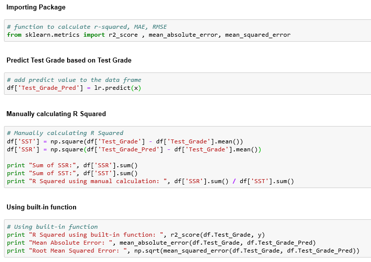
R-Squared for Goodness of Fit:

The R-squared metric is the most popular practice of evaluating how well your model fits the data. R-squared value designates the total proportion of variance in the dependent variable explained by the independent variable. It is a value between 0 and 1; the value toward 1 indicates a better model fit. See the table below.

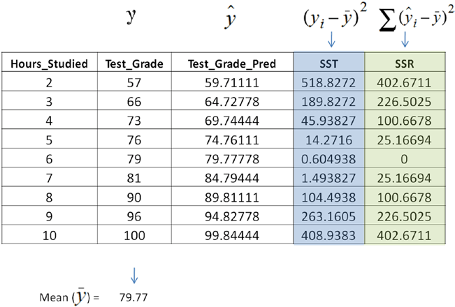
Where,

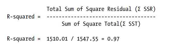
In this case R-squared can be interpreted as 97% of variability in the
dependent variable (test score) can be explained by the independent variable (hours studied).

Root Mean Squared Error (RMSE):

This is the square root of the mean of the squared errors. RMSE indicates how close the predicted values are to the actual values; hence a lower RMSE value signifies that the model performance is good. One of the key properties of RMSE is that the unit will be the same as the target variable.

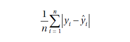
Mean Absolute Error:

This is the mean or average of absolute value of the errors, that is, the predicted – actual.

Linear regression model accuracy matrices:

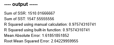
Multiple Linear Regression

Multiple linear regression:
One quantitative dependent variable
Many quantitative independent variables

Multiple linear regression is the most common form of linear regression analysis.  As a predictive analysis, the multiple linear regression is used to explain the relationship between one continuous dependent variable and two or more independent variables.  

lets do some programming on Multiple Linear Regression:

1. Import the libraries:
2. Load the dataset and extract independent and dependent variables:
3. Finding the correlation in dataset.
4. Encoding the categorical data:
5. Avoid dummy variable trap.
6. Splint the data into train and test set.
7. Fitting multiple linear regression models to training set.
8. Predict Test set result.
9. Calculating the coefficients and intercepts.
10. Evaluating the model.

1. Import the libraries:

# Importing the libraries
import numpy as np
import matplotlib.pyplot as plt
import pandas as pd
import seaborn as sns

from sklearn.preprocessing import LabelEncoder, OneHotEncoder
from sklearn.model_selection import train_test_split
from sklearn.linear_model import LinearRegression
from sklearn.metrics import r2_score

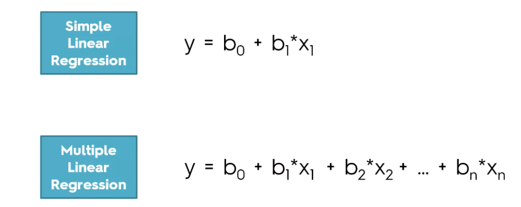
2. Load the dataset and extract independent and dependent variables:

# Importing the dataset
df = pd.read_csv('../Data/50_Companies.csv')
X = df.iloc[:, :-1].values
y = df.iloc[:, 4].values
df.head()

3. Finding the correlation in dataset:

sns.heatmap(df.corr(), annot=True)

4. Encoding the categorical data:

Problem with Categorical Data and how to convert this to Numerical Data?

Many machine learning algorithms cannot operate on label data directly. They require all input variables and output variables to be numeric.

Converting categorical data into numerical data involves two steps:

1. Integer Encoding
   • Each unique category value is assigned an integer value. For example, “red” is 1, “green” is 2, and “blue” is 3. This is called a label encoding or an integer encoding and is easily reversible.
2. One-Hot Encoding
   • This will convert n levels to n-1 new variable,
     and the new variables will use 1 to indicate the presence of level
     and 0 for otherwise. Note that before calling OneHotEncoder,
     we should use LabelEncoder to convert levels to number.

# Encode labels with value between 0 and n_classes-1.
labelencoder = LabelEncoder() 

# Fit label encoder and return encoded labels
X[:, 3] = labelencoder.fit_transform(X[:, 3]) 

# Encode categorical integer features as a one-hot numeric array.
onehotencoder = OneHotEncoder(categorical_features = [3]) 

# Fit OneHotEncoder to X, then transform X.
X = onehotencoder.fit_transform(X).toarray() 

5. Avoid dummy variable trap:

# Avoiding the Dummy Variable Trap
X = X[:, 1:]

6. Split the data into train and test set:

# Split train and test data, test size is 20%.
X_train, X_test, y_train, y_test = train_test_split(X, y, test_size = 0.20, random_state = 1)

7. Fitting multiple linear regression models to training set:

regressor = LinearRegression()
regressor.fit(X_train, y_train)

8. Predict Test set result:

y_pred = regressor.predict(X_test)
y_pred

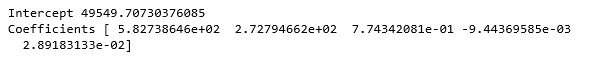
9. Calculating the coefficients and intercepts:

# Calculating the Intercept
print("Intercept", regressor.intercept_)

# Calculating the Coefficients
print("Coefficients", regressor.coef_)

10. Evaluating the model:

# R^2 (coefficient of determination) regression score function
# Best possible score is 1.0, lower values are worse.
r2_score(y_test, y_pred)

— Output —-

0.9649618042060571

References:

1. Book: Mastering Machine Learning with Python by Manohar Swamynathan.
2. Udemy course on Machine Learning A-Z™: Hands-On Python & R In Data Science at link.
3. Glossary – Statistics by Jim at link.

To be continued..