Purnananda Behera

What is Data Dimensionality?

In real world, number of columns is the number of dimensions of data.However, some columns are similar, some are correlated, some are duplicates in some way, some are junk, some are useless, etc. so the actual number of dimensions can be unknown. Its a knotty problem.

What is high dimensionality?

Suppose we have 500 variables in a data set. As it a very huge number, so it is quite difficult to read and understand the data. This is known as high dimensionality. Anything which can’t be read and understood without any use of external resources is an example of high dimensionality.

What is PCA?

Principal Component Analysis, or PCA, is a dimensionality-reduction method that is often used to reduce the dimensionality of large data sets, by transforming a large set of variables into a smaller one that still contains most of the information in the large set.

Reducing the number of variables of a data set naturally comes at the expense of accuracy, but the trick in dimensionality reduction is to trade a little accuracy for simplicity. Because smaller data sets are easier to explore and visualize and make analyzing data much easier and faster for
machine learning algorithms without extraneous variables to process.

So to sum up, the idea of PCA is simple — reduce the number of variables of a data set, while preserving as much information as possible.

Basically PCA is a dimension reduction methodology that aims to reduce a large set of (often correlated) variables into a smaller set of (uncorrelated) variables, called principal components, which holds sufficient information without losing the relevant info much.

Somewhat unsurprisingly, reducing the dimension of the feature space is called “dimensionality reduction.” There are many ways to achieve dimensionality reduction, but most of these techniques fall into one of two classes:

• Feature Elimination
• Feature Extraction

Feature elimination is what it sounds like: we reduce the feature space by eliminating features. Advantages of feature elimination methods include simplicity and maintaining interpretability of your variables.

As a disadvantage, we’re missing out on whatever the dropped variables could contribute to our model. By eliminating features, we’ve also entirely eliminated any benefits those dropped variables would bring.

Feature extraction however, doesn’t run into this problem. Say we have ten independent variables. In feature extraction, we create ten “new” independent variables, where each “new” independent variable is a combination of each of the ten “old” independent variables.
However, we create these new independent variables in a specific way and order these new variables by how well they predict our dependent variable.

You might say, “Where does the dimensionality reduction come into play?” Well, we keep as many of the new independent variables as we want, but we drop the “least important ones.” Because we ordered the new variables by how well they predict our dependent variable, we know which variable is the most important and least important. But — and here’s the kicker — because these new independent variables are combinations of our old ones, we’re still keeping the most valuable parts of our old variables, even when we drop one or more of these “new” variables!

Principal component analysis is a technique for feature extraction — so it combines our input variables in a specific way, then we can drop the “least important” variables while still retaining the most valuable parts of all of the variables! As an added benefit, each of the “new” variables after PCA are all independent of one another. This is a benefit because the assumptions of a linear model require our independent variables to be independent of one another. If we decide to fit a linear regression model with these “new” variables (see “principal component regression” below), this assumption will necessarily be satisfied.

When should I use PCA?

• Do you want to reduce the number of variables, but aren’t able to identify variables to completely remove from consideration?
• Do you want to ensure your variables are independent of one another?
• Are you comfortable making your independent variables less interpretable?

If you answered “yes” to all three questions, then PCA is a good method to use. If you answered “no” to question 3, you should not use PCA.

How does PCA work?

• Dimensionality It is the number of random variables in a dataset or simply the number of features, or rather more simply, the number of columns present in your dataset.

• Correlation It shows how strongly two variable are related to each other. The value of the same ranges for -1 to +1. Positive indicates that when one variable increases, the other increases as well, while negative indicates the other decreases on increasing the former. And the modulus value of indicates the strength of relation.

• Orthogonal: Uncorrelated to each other, i.e., correlation between any pair of variables is 0.

• Eigenvectors: Eigenvectors and Eigenvalues are in itself a big domain, let’s restrict ourselves to the knowledge of the same which we would require here. So, consider a non-zero vector v. It is an eigenvector of a square matrix A, if Av is a scalar multiple of v. Or simply:

Av = ƛv
Here, v is the eigenvector and ƛ is the eigenvalue associated with it.

• Covariance Matrix: This matrix consists of the covariances between the pairs of variables. The (i,j)th element is the covariance between i-th and j-th variable.

PCA as a whole

Python Code (PCA on Iris dataset)

Import required modules:

import numpy as np
import pandas as pd
from sklearn.decomposition import PCA
import seaborn as sns

sns.set(style="whitegrid")

Get the data:

path = "https://archive.ics.uci.edu/ml/machine-learning-databases/iris/iris.data"
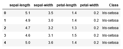
headernames = ['sepal-length', 'sepal-width', 'petal-length', 'petal-width', 'Class']
df = pd.read_csv(path, names = headernames)
df.head()

Now use PCA for dimensionality reduction of the iris dataset, retaining only the 2 most important components

# Create a PCA model with 2 components: pca
pca = PCA(n_components = 2)

# Fit the PCA instance to the scaled samples
pca.fit(df.iloc[:,0:4])

# Transform the scaled samples: pca_features
pca_features = pca.transform(df.iloc[:,0:4])

# Print the shape of pca_features
print(pca_features.shape)

(150, 2)

explained_variance_ratio_: Percentage of variance explained by each of the selected components.

How can we be sured that numbers of PCA components required?

Ans: If the explained_variance_ratio_ >= 90% or more, then we will be sured that we are covering the data in better sense.

pca.explained_variance_ratio_

array([0.92461621, 0.05301557])

pca.explained_variance_ratio_.cumsum()

array([0.92461621, 0.97763178])

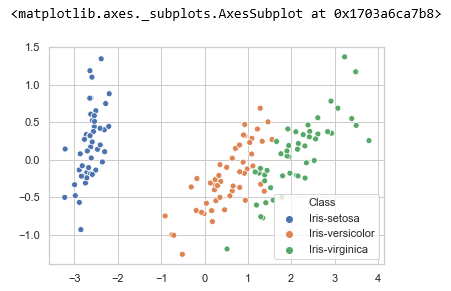
let us represent the data using scatter plot.

xs = pca_features[:,0]
ys = pca_features[:,1]

sns.scatterplot(x=xs, y=ys, hue=df.iloc[:,-1])

References:

Link 1: https://hackernoon.com/dimensionality-reduction-using-pca-a-comprehensive-hands-on-primer-ph8436lj

Link 2: https://github.com/Mathanraj-Sharma/sample-for-medium-article/blob/master/PCA-Example