Purnananda Behera

A classification problem has a discrete value as its output.

For example, “likes pineapple on pizza” and “does not like pineapple on pizza” are discrete.

ML Mind Map:

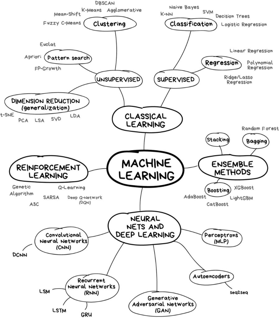
What is a K-Nearest Neighbor Algorithm (KNN)?

KNN is one of the simplest classification algorithms and it is one of the most used learning algorithms.

KNN is a simple algorithm that stores all available cases and classifies new cases based on a similarity measure (eg distance function).

KNN is based on feature similarity.

Real-Life Example

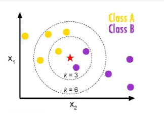
belongs to the yellow family and Class B is belonged to the purple class according to the above figure. Then train dataset in KNN model which we discuss later but focus on just example here k=3 is three nearest neighbors a k=6 six nearest neighbors. so when we take k=3 then what happens and when k=6 then what happens. When k=3 then two belong to a purple class and one belongs to the yellow class majority vote of purple so here the purple class is considered similarly when k=6 then four belong to a yellow class and two belong to purple class so majority votes are yellow so consider the yellow class. So in this way KNN works.

The KNN algorithm itself is fairly straightforward and can be summarized by the following steps:

1. Choose the number of k and a distance metric.
2. Find the k nearest neighbors of the sample that we want to classify.
3. Assign the class label by majority vote.
4. K must be odd always.

How k-Nearest Neighbor Algorithm Works?

The KNN algorithm works based on the similarity instances. The similarity is defined according to a distance metric between two data points.

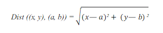
A popular choice is a Euclidean distance very often.

According to the Euclidean distance formula, the distance between two points in the plane with coordinates (x, y) and (a, b) is given by:

KNN runs through the whole dataset computing d between x and each training observation. We’ll call k points in the training dataset to x the set A. Note that k is usually odd to prevent a situation.

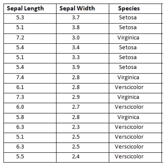
Dataset:

This dataset is about Iris was taken from the UCI Repository. In this dataset, we have 3 attributes which have sepal length, sepal width, and species. Species have a target attribute. In target attribute, we have three species (Setosa, Virginia, and Versicolor) and our target finds the nearest species which belong from three species using the k-Nearest Neighbors.

Target: New flower found, need to classify “Unlabeled”.

Feature of the new unlabeled flower:

Solution:

Step 1: Find Distance:

Our first step is to find distance using the Euclidean distance between Actual and Observed sepal length and sepal width. For the first instance dataset.

X = Observed sepal length=5.2

Y = Observed sepal width=3.1

Now Actual which is given in the dataset

A = Actual sepal length = 5.3

B = Actual sepal width=3.7

Distance formula:

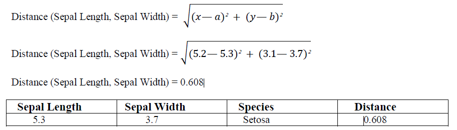
This is for first instances which I find the distance similarly find all the remaining instances distance as shown below in the table.

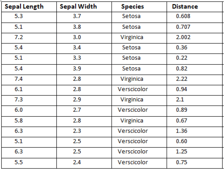
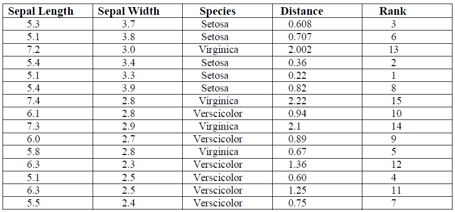
Step 2: Find Rank:

In this step, we find the Rank after finding the Distance. Rank basically gives the number according to ascending order distance. As you can see below table:

If we see the above table then instance number 5 has a minimum distance 0.22 so gave him rank as below table.

Similarly, find the rank for all other instances as shown below the table.

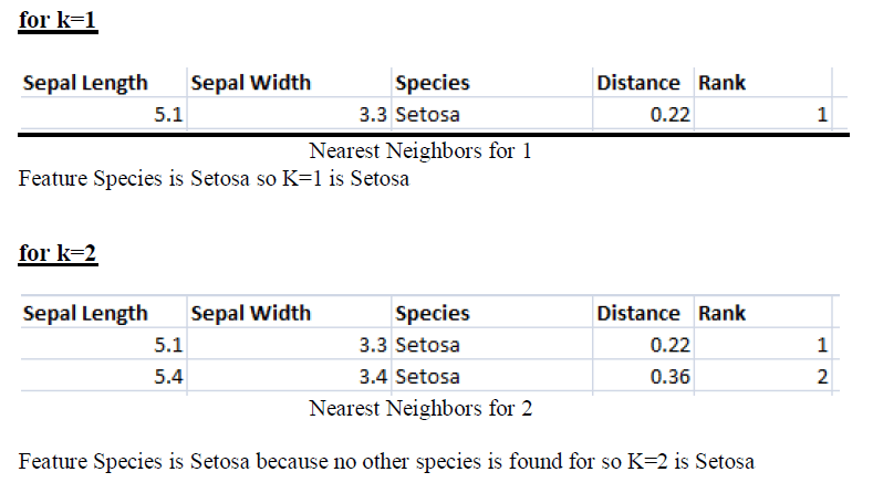
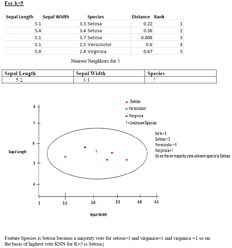
Step 3: Find the Nearest Neighbor:

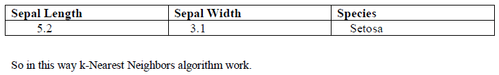
Our last step finds the nearest neighbors on the basis of distance and rank we can find our Unknown on the basis of species. According to rank find the k Nearest Neighbor.

Implementing KNN algorithm with Python

import numpy as np
import pandas as pd
import matplotlib.pyplot as plt

path = "https://archive.ics.uci.edu/ml/machine-learning-databases/iris/iris.data"
headernames = ['sepal-length', 'sepal-width', 'Class']

df = pd.read_csv(path, names = headernames)
df.head()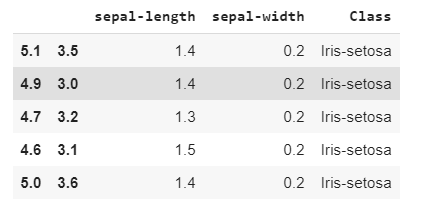

Data Preprocessing will be done with the help of following script lines.

# create design matrix X and target vector y
X = df.iloc[:, :-1].values
y = df.iloc[:, 2].values

Next, we will divide the data into train and test split. Following code will split the dataset into 75% training data and 25% of testing data:

from sklearn.model_selection import train_test_split

# split into train and test
X_train, X_test, y_train, y_test = train_test_split(X, y, test_size = 0.25)

Next, data scaling will be done as follows:

from sklearn.preprocessing import StandardScaler

scaler = StandardScaler()
scaler.fit(X_train)
X_train = scaler.transform(X_train)
X_test = scaler.transform(X_test)

Next, train the model with the help of KNeighborsClassifier class of sklearn as follows:

from sklearn.neighbors import KNeighborsClassifier

# instantiate learning model (k = 3)
classifier = KNeighborsClassifier(n_neighbors = 3)

# fitting the model
classifier.fit(X_train, y_train)

At last we need to make prediction. It can be done with the help of following script:

# predict the response
y_pred = classifier.predict(X_test)

Next, print the results as follows:

from sklearn.metrics import classification_report, confusion_matrix, accuracy_score

# validate the prediction result.
result = confusion_matrix(y_test, y_pred)
print("Confusion Matrix:")
print(result)

print("\n")

# evaluate the prediction report.
result1 = classification_report(y_test, y_pred)
print("Classification Report:",)
print (result1)

# evaluate accuracy.
result2 = accuracy_score(y_test, y_pred)
print("Accuracy:", result2)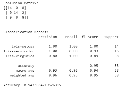

Let’s check the accuracy for various values of n for K-Nearest neighbors.

#for checking the model accuracy
from sklearn import metrics 

a_index=list(range(1,11))
a=pd.Series()
x=[1,2,3,4,5,6,7,8,9,10]

for i in list(range(1,11)):
    model=KNeighborsClassifier(n_neighbors=i) 
    model.fit(X_train,y_train)
    prediction=model.predict(X_test)
    a=a.append(pd.Series(metrics.accuracy_score(prediction,y_test)))

plt.plot(a_index, a, marker="o")
plt.xticks(x)
plt.title("Accuracy vs K Value")
plt.xlabel("K")
plt.ylabel("Accuracy")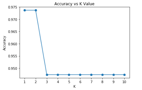

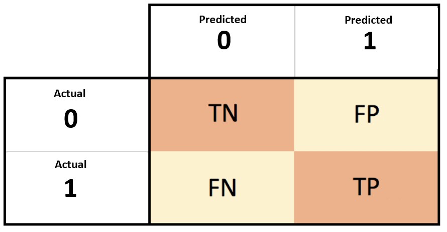
Confusion Matrix:

• A confusion matrix is a summary of prediction results on a classification problem.
• The confusion matrix shows the ways in which your classification model is confused when it makes predictions.

Confusion Matrix Case Study

Let’s pretend we have a two-class classification problem of predicting whether a photograph contains a man or a woman.

We have a test dataset of 10 records with expected outcomes and a set of predictions from our classification algorithm.

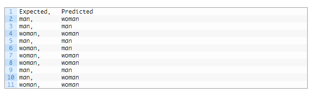
Let’s start off and calculate the classification accuracy for this set of predictions.

The algorithm made 7 of the 10 predictions correct with an accuracy of 70%.

But what type of errors were made?

Let’s turn our results into a confusion matrix.

First, we must calculate the number of correct predictions for each class.

Now, we can calculate the number of incorrect predictions for each class, organized by the predicted value.

We can now arrange these values into the 2-class confusion matrix:

This gives us:

• “true positive” for correctly predicted event values.
• “false positive” for incorrectly predicted event values.
• “true negative” for correctly predicted no-event values.
• “false negative” for incorrectly predicted no-event values.

Classification Report:

A Classification report is used to measure the quality of predictions from a classification algorithm. How many predictions are True and how many are False.

Accuracy:

• Accuracy refers to how close a measurement is to the true value.
• Accuracy Formula: (TP+TN)/(TP+TN+FP+FN)
• where: TP = True positive; FP = False positive; TN = True negative; FN = False negative.

Error rate:

• The inaccuracy of predicted output values is termed the error of the method.
• Error rate formula: (False Positive + False Negative) / Total
• Also we can say error rate = 1 – Accuracy.

Precision:

• What proportion of positive identifications was actually correct?
• Precision Formula: True Positive / (True Positive + False Positive)
• Precision in simple terms: What percent of positive prediction made were correct?
• For example: 3 predictions are correct out of 4. In that case precision will be 3/4 is equal to .75.

Recall:

• What proportion of actual positives was identified correctly?
• Recall in simple terms: What percent of actual positive values were correctly classified by your classifier?
• Recall Formula: True Positive / (True Positive + False Negative)

F Score:

• F1 score is a weighted average score of the true positive (recall) and precision.
• F1 Score Formula: 2x(Recall x Precision) / (Recall + Precision)

Support:

• The support is the number of occurrence of the given class in your dataset.
• The support is the number of occurrences of each class in y_true.

KNN Pros and Cons:

Pros:

1. Very simple to use.
2. Works with any number of classes.
3. Easy to add more data.
4. Very few parameters: K, Distance Metric

Cons:

1. High prediction cost (Worse for large data sets)
2. Not goo with high dimensional data.
3. Categorical features don’t work well.

References:

1. Blog: Confusion Matrix by Link
2. Paper: An Intuitive Guide of K-Nearest Neighbor with Practical Implementation in Scikit Learn.
3. Udemy: Python-for-data-science-and-machine-learning-bootcamp

To be continued..