Predicting Wine Quality using different classifiers

In this blog, we have done some data exploration using matplotlib and seaborn.

Here we have used three different classifier models to predict the wine quality:

K-Nearest Neighbors Classifier
Support Vector Classifier
Random Forest Classifier

Also we have classified wine qualities into 3 different categories as good, average and bad.

Dataset Information:

The two datasets are related to red and white variants of the Portuguese “Vinho Verde” wine.

Attribute information:

Input variables (based on physicochemical tests):
1 – fixed acidity
2 – volatile acidity
3 – citric acid
4 – residual sugar
5 – chlorides
6 – free sulfur dioxide
7 – total sulfur dioxide
8 – density
9 – pH
10 – sulphates
11 – alcohol Output variable (based on sensory data)
12 – quality (score between 0 and 10)

Dataset URL: http://mlr.cs.umass.edu/ml/machine-learning-databases/wine-quality/winequality.names

let’s start writing python code for the predictor we are going to build.

Import required modules:

import numpy as np
import pandas as pd
import matplotlib.pyplot as plt
import seaborn as sns
%matplotlib inline

Get the data:

dataset_url = 'http://mlr.cs.umass.edu/ml/machine-learning-databases/wine-quality/winequality-red.csv'
data = pd.read_csv(dataset_url, sep=';')
data.head()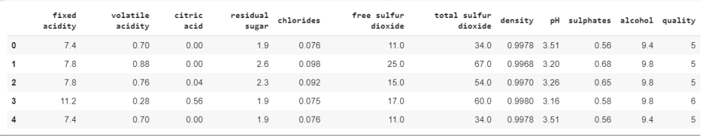

Lets’s check any missing values exist in the data collection.

data.isnull().values.any()

Output: False

Create a new feature as category to classify the wine quality

quality = data["quality"].values
category = []
for num in quality:
    if num<5:
        category.append("Bad")
    elif num>6:
        category.append("Good")
    else:
        category.append("Average")

#Create a new feature for wine category.
category = pd.DataFrame(data=category, columns=["category"])
data = pd.concat([data,category],axis=1)

Let’s explore the data

In this section we will be doing some exploratory data analysis to have a better understanding of the data we are working with.

plt.figure(figsize=(6,4))
sns.countplot(data["category"], palette="Reds")

Check the correlation for each fields:

plt.figure(figsize=(12,8))
sns.heatmap(data.corr(),annot=True)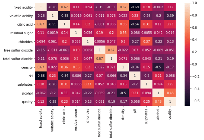

According to heatmap, we can focus on alcohol, sulphates, density, and quality relations to get meaningful insight.

Let’s draw the pairplot to see the data distribution for above highlighted features.

sns.pairplot(data, vars=["alcohol", "density", "sulphates"], hue="category", markers=["o", "s", "D"])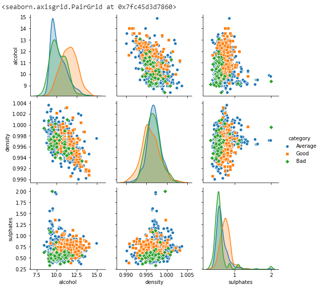

Find the relationship between density and alcohol.

plt.figure(figsize=(12,6))
sns.jointplot(y=data["density"],x=data["alcohol"],kind="hex")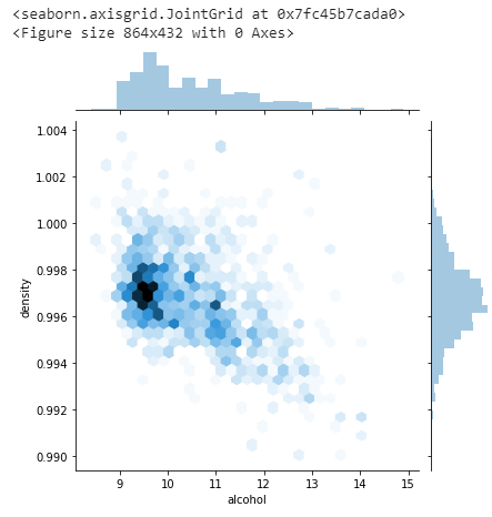

Explore the Quality data distribution.

sns.countplot(x='quality', data=data, palette="Reds")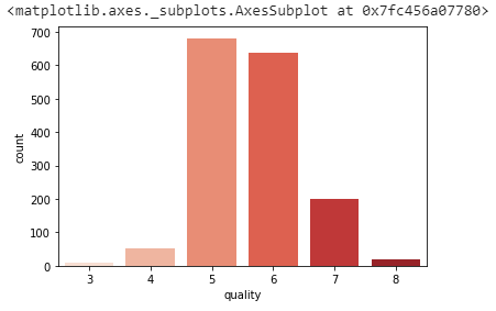

Find the relationship between alcohol and quality.

plt.figure(figsize=(8,5))
sns.barplot(x=data["quality"],y=data["alcohol"],palette="Reds")

Extracting relevant features for data processing.

headerNames = ['alcohol', 'density', 'sulphates', 'category']
df = data[headerNames]
df.head()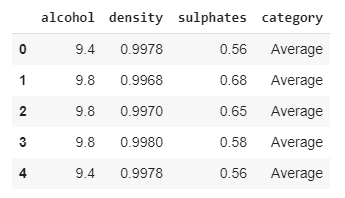

Data Preprocessing will be done with the help of following script lines.

# create design matrix X and target vector y
X = df.iloc[:, :-1].values
y = df.iloc[:, -1].values
print(np.unique(y))

Output: [‘Average’ ‘Bad’ ‘Good’]

We have used, train_test_split() function that we imported from sklearn to split the data. Notice we have used test_size=0.25 to make the test data 25% of the original data. The rest 80% is used for training.

from sklearn.model_selection import train_test_split

# split into train and test
X_train, X_test, y_train, y_test = train_test_split(X, y, test_size = 0.25)

Here we will use standardscalaer() function from sklear library to normalize the values to improve the model accuracy.

from sklearn.preprocessing import StandardScaler

scaler = StandardScaler()
scaler.fit(X_train)
X_train = scaler.transform(X_train)
X_test = scaler.transform(X_test)

This function will be use to print the classification report.

from sklearn.metrics import classification_report, confusion_matrix, accuracy_score

def print_classification_report(title, y_test, y_pred):
  '''
  This function is used to print the classification report.
  '''

  print(title + " \n")

  # validate the prediction result.
  result = confusion_matrix(y_test, y_pred)
  print("Confusion Matrix:")
  print(result)

  print("\n")

  # evaluate the prediction report.
  result1 = classification_report(y_test, y_pred)
  print("Classification Report:",)
  print (result1)

  # evaluate accuracy.
  result2 = accuracy_score(y_test, y_pred)
  print("Accuracy:", result2)

Create two variables to capture the accuracy of different models.

models = []
accuracies = []

Implement K-Nearest Neighbors Classifier

from sklearn.neighbors import KNeighborsClassifier

# instantiate learning model (k = 8)
knn = KNeighborsClassifier(n_neighbors = 8)

# fitting the model
knn.fit(X_train, y_train)

# predict the response
y_pred = knn.predict(X_test)

# Capture the accuracy score.
# accuracy_dict.__setitem__("KNN", accuracy_score(y_test, y_pred))
models.append("KNN")
accuracies.append(accuracy_score(y_test, y_pred))

# Print the classification report.
print_classification_report("K-Nearest Neighbors Classifier Report:", y_test, y_pred)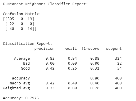

Implement Random Forest Classifier

from sklearn.ensemble import RandomForestClassifier

# instantiate learning model
rfc = RandomForestClassifier(n_estimators=250)

# fitting the model
rfc.fit(X_train, y_train)

# predict the response
y_pred = rfc.predict(X_test)

# Capture the accuracy score.
# accuracy_dict.__setitem__("Random Forest", accuracy_score(y_test, y_pred))
models.append("Random Forest")
accuracies.append(accuracy_score(y_test, y_pred))


# Print the classification report.
print_classification_report("Random Forest Classifier Report:", y_test, y_pred)

Implement Support Vector Machine Classifier

from sklearn.svm import SVC

# instantiate learning model
svc = SVC()

# fitting the model
svc.fit(X_train,y_train)

# predict the response
y_pred =svc.predict(X_test)

# Capture the accuracy score.
# accuracy_dict.__setitem__("SVM", accuracy_score(y_test, y_pred))
models.append("SVM")
accuracies.append(accuracy_score(y_test, y_pred))

# Print the classification report.
print_classification_report("Support Vector Machine Classifier Report:", y_test, y_pred)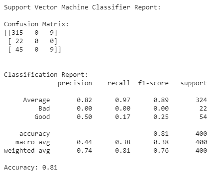

Wrapping it up

Its time to compare the model accuracy.

report = pd.DataFrame({'model': models, 'accuracy': accuracies})
report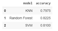

This gives us the accuracy above 80% using above three classifiers models. Overall our predictor performs quite well, in-fact any accuracy % greater than 80% is considered as great.

If we choose one out of all these classifiers, then Random Forest accuracy is 82% which quite better than others.

If you find this blog useful then please like this page.

References:

Dataset Information: http://mlr.cs.umass.edu/ml/machine-learning-databases/wine-quality/winequality.names

Purnananda Behera